Introduction

DL vs ML

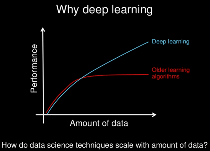
Deep learning is an evolution of traditional Machine Learning. The more high-quality data we have, the better deep learning algorithms will perform. This is not always the case for traditional ML, which can stagnate after a certain level.

Deep learning is based on Artificial Neural Networks (ANN), inspired by how the human brain works.

ML: Linear regression / Decision trees
DL: Artificial Neural Networks (ANN)

ANNs can capture deeper patterns than traditional ML. Deep learning uses multiple layers; the more layers, the deeper the learned representation — hence the name "Deep Learning".

Deep learning typically requires significant compute power.

Perceptron

Neural networks are built from layers. Each layer takes inputs and applies parameters to produce outputs.

A single neuron (perceptron) has: a weight vector $w$, a bias $b$, and an activation function $f$.

Dot product: $$ w^\top x \,=\, \sum_{j=1}^{n} w_j x_j $$

Perceptron output for an input $x$: $$ h \,=\, f(w^\top x + b) $$

The perceptron is a linear model, most effective when data can be linearly separated.

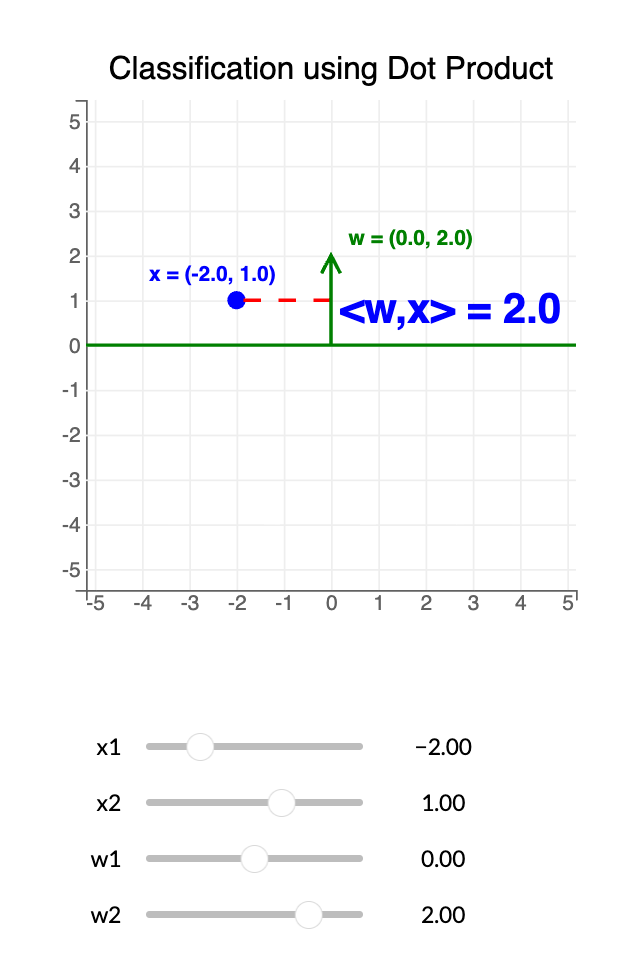
Dot product

For a point $x = (x_1, x_2)$ and a vector $w = (w_1, w_2)$:

• If $w^\top x > 0$ → class 1
• If $w^\top x < 0$ → class 0

The decision boundary is $w^\top x = 0$, separating positive from negative.

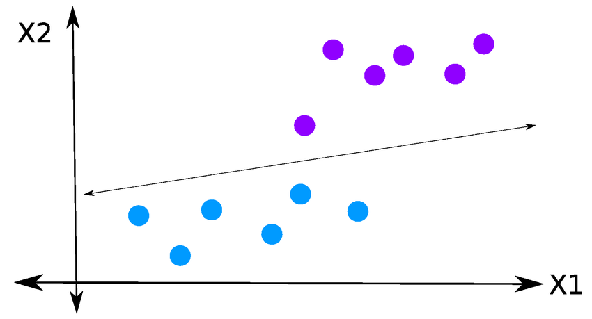
Linear separability

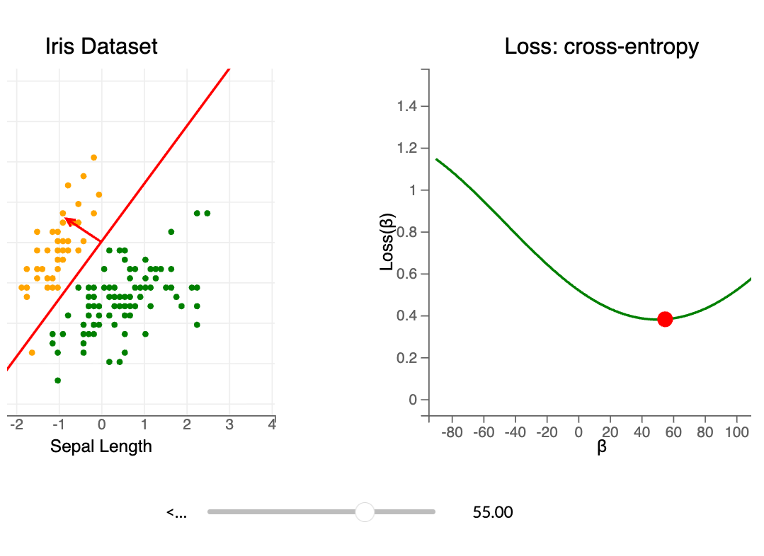
To use dot products for classification, linear separability matters. Example: the Iris dataset using Sepal Width and Sepal Length.

Goal: find a decision boundary to separate species (Green: Iris setosa, Orange: Iris virginica).

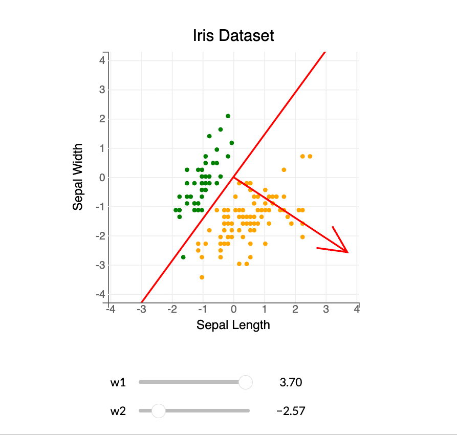
Separating hyperplane: $$ \{ x \in \mathbb{R}^2 : \langle x, w \rangle = x_1 w_1 + x_2 w_2 = 0 \} $$

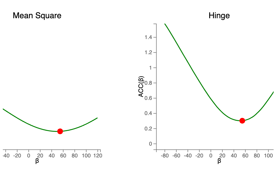
Loss function

We count classification errors for a given $w$.

Given $n$ points $X = (x_i)_{i=1,\dots,n} \in \mathbb{R}^d$ and labels $Y = (y_i)_{i=1,\dots,n} \in \{0,1\}$.

Classifier: $$ f(x_i, w) = \mathbf{1}[\langle x_i, w \rangle \ge 0] $$

Empirical 0/1 loss: $$ g(w,X,Y) = \sum_{i=1}^{n} \mathbf{1}[ f(x_i, w) \ne y_i ] $$

We minimize this loss to find the best separating hyperplane.

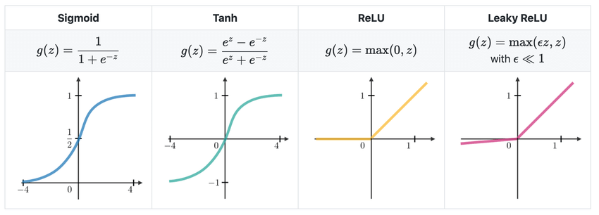
Activation function

Activation functions enable differentiable loss and appropriate outputs.

• Sigmoid
• Tanh
• ReLU (Rectified Linear Unit)
• Leaky ReLU

Hidden layers: often ReLU / Leaky ReLU.

Output layer depends on task: binary → Sigmoid; multiclass → Softmax; regression → Linear.

Gradient descent

With differentiable activations, we can use gradient descent to optimize $w$.

Example: if $f(x)=x^2$, then $f'(x)=2x$.

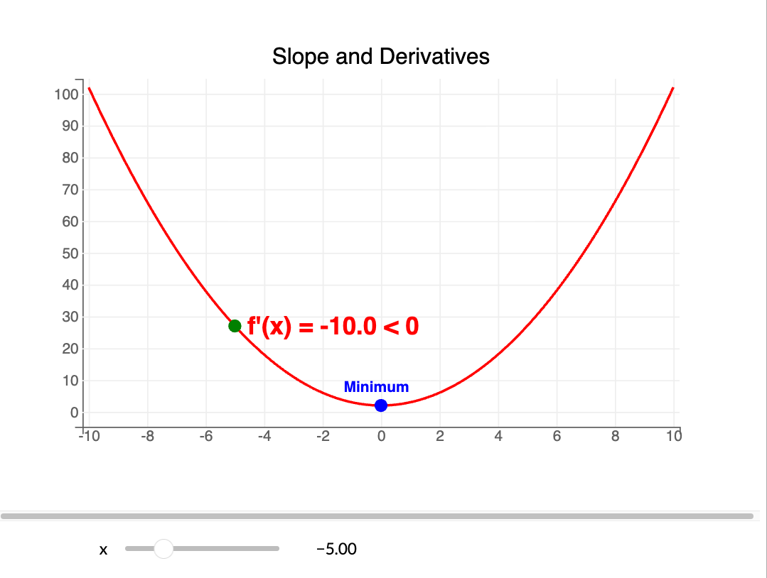
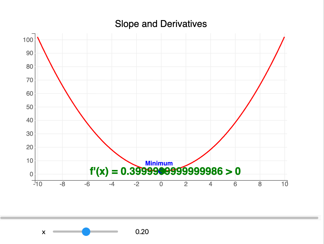
Learning rate $\\lambda$ controls step size. Iterate until $|f'(x_k)| < {tol}$.

Update rule: $$ x_{k+1} = x_k - \lambda f'(x_k) $$

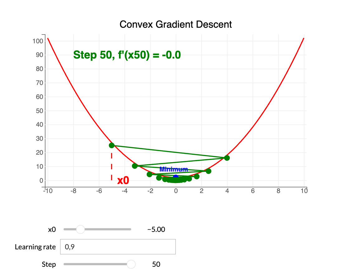
Limitations: guarantees a global minimum only for convex functions. In DL, loss is non-convex; gradient methods often reach a local minimum.

Therefore, the learning rate is a critical hyperparameter for DL model performance.

Predictions with neural networks on tabular data

Context

We will train a multilayer perceptron on the Iris dataset (3 species). The goal is to classify the species from tabular features.

Multilayer perceptron (MLP)

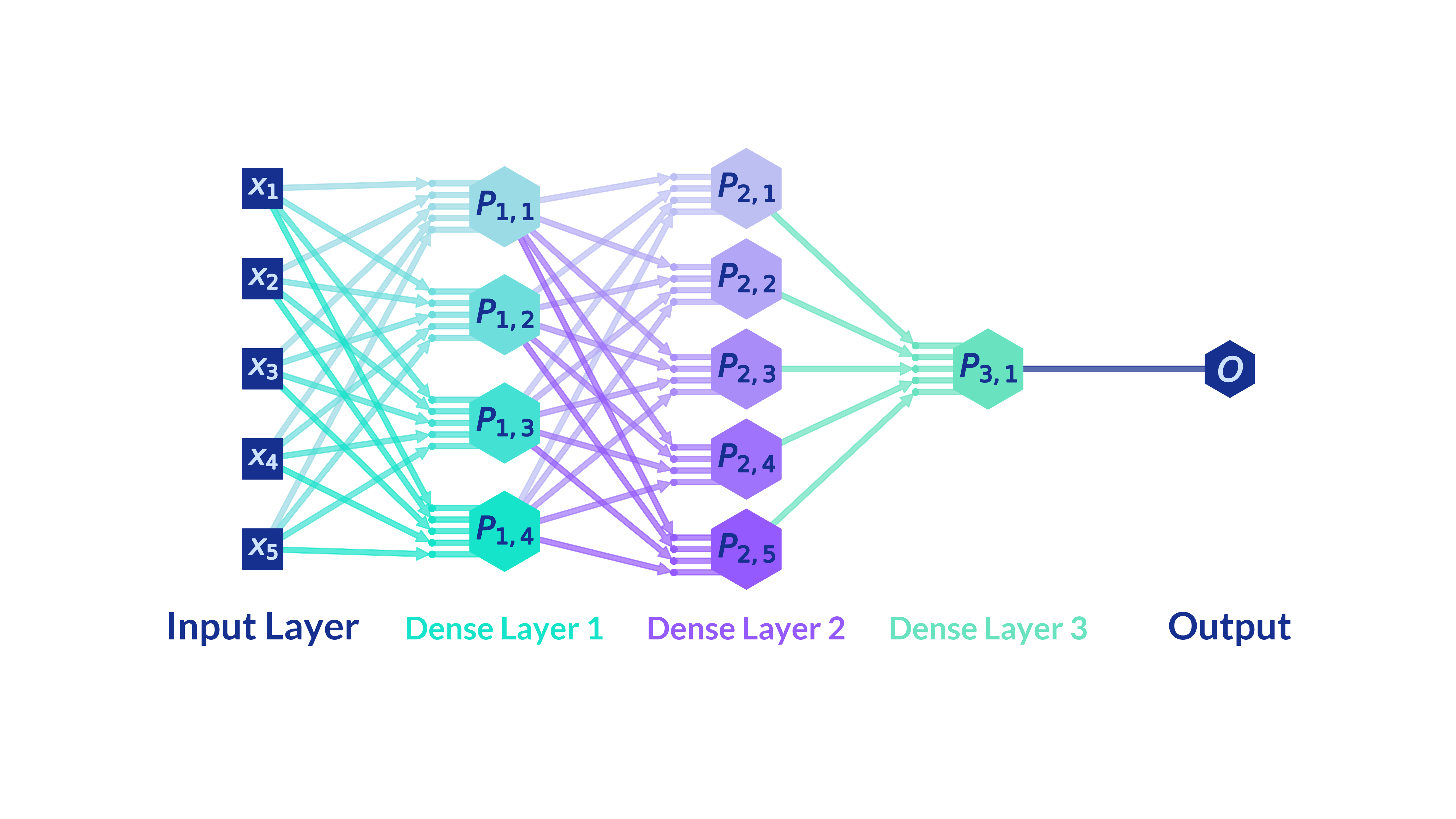
An MLP is a sequence of layers where each layer’s input is the previous layer’s output. For three layers and input $x$:

$$ H_1 = \text{Layer}_1(x),\quad H_2 = \text{Layer}_2(H_1),\quad O = \text{Layer}_3(H_2). $$

API styles:

• Sequential: linear stack of layers (simple networks)
• Functional: flexible graphs (multiple inputs/outputs, merges)

Training pipeline

1. Architecture definition: choose number of layers/neurons and data flow
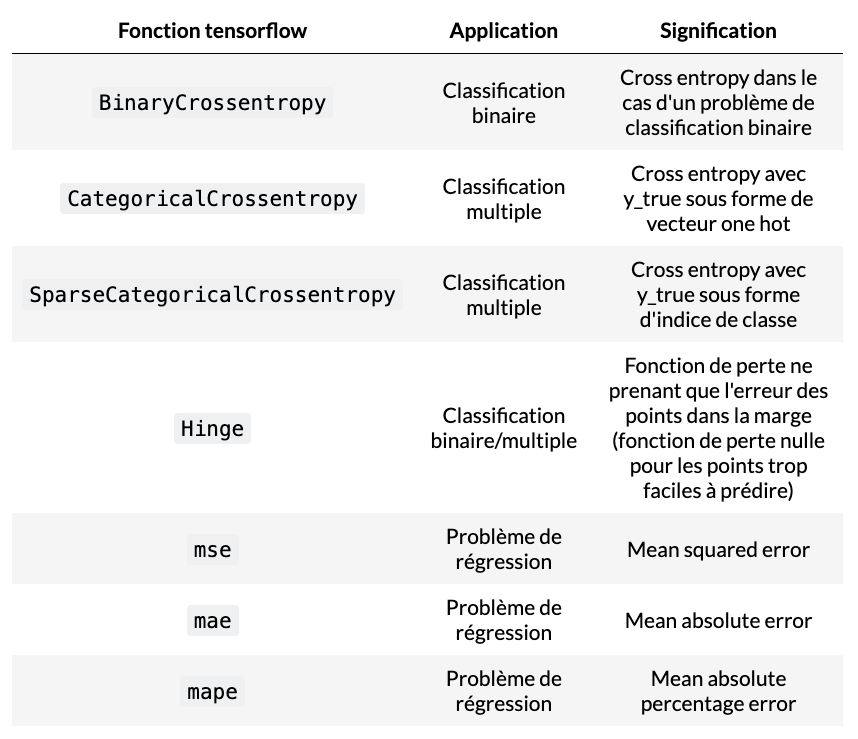
2. Compilation: loss, metrics, optimizer (e.g., Adam)

model.compile(
    loss="name_loss_function",
    optimizer="name_optimizer",
    metrics=["name_metric"],
)
        

3. Training: run fit across epochs

model.fit(
    X_train, y_train,
    validation_split=p,
    epochs=nb_epochs,
    batch_size=batch_size,
)
        

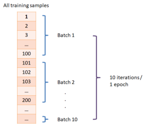
Key notions: batch_size (samples per update); batch → model → prediction → loss → weight update; epochs (full passes over data).

validation_split holds out a portion of training data; evaluation runs at each epoch end.

Sequential model with Keras

from tensorflow.keras.models import Sequential
from tensorflow.keras.layers import Dense

model = Sequential()
model.add(Dense(units=64, activation="relu", input_shape=(784,)))
model.add(Dense(units=10, activation="softmax"))

model.fit(X, y, epochs=nb_epochs, batch_size=batch_size, validation_split=p)
        

Model performance

Use a confusion matrix on the test set. Convert probabilities to class IDs with NumPy argmax for scikit‑learn reports. For multi‑class tasks, a common loss is sparse_categorical_crossentropy.